
It’s been quite a while since I wrote about my favorite application, Microsoft Excel. When I’m not using different combinations of formulas and applying beautiful styles to my spreadsheets, I find that there are many fantastic tools within Excel that many people have never used. These tools aren’t actually hidden, but if you don’t know what you’re looking for, you can easily miss them. Here are my seven favorite Excel tools that you can start using today.
1. Freeze Top Row
This is a fairly well known tool, but I still often find people who don’t know it exists. When you have a spreadsheet with enough data that you are required to scroll, have you ever wished that you could still see the top row that has the headings?
There are two ways to solve this. The first is to format your data as a table. When you do this, you identify the data as a collection or database. Excel will automatically make the top row the headers for each column when you scroll. To make this happen, go to Home > Format as Table, and select any style.
The other way to keep the top row always visible is to actually freeze it. To do this, go to View > Freeze Panes > Freeze Top Row.

2. Drop-Down Lists with Data Validation
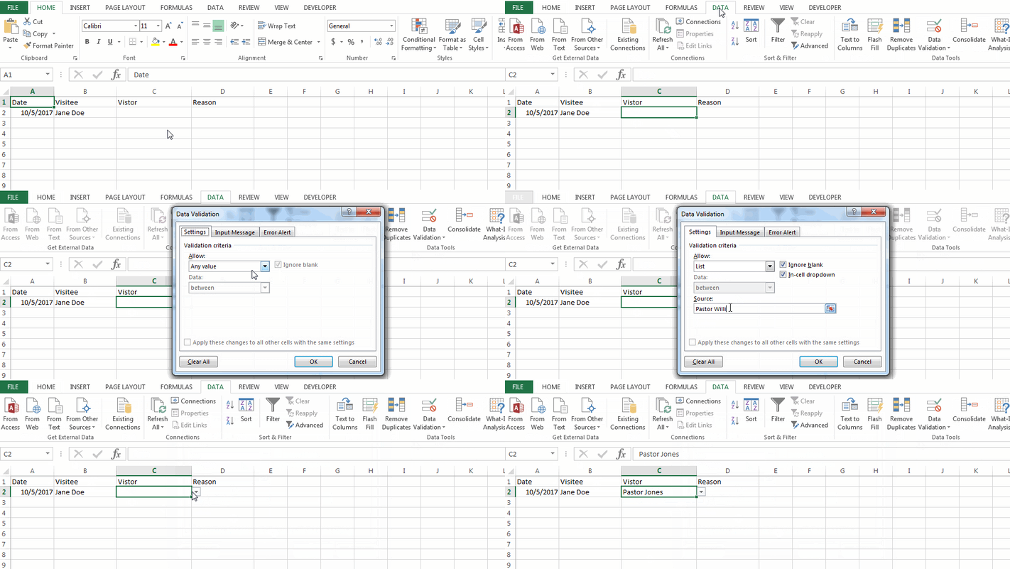
Consistent data entry is crucial in whatever work you do, but especially in spreadsheets. I use Data Validation to build drop-down lists within cells so when I go to enter data into a cell, I can only use the options in that drop-down list. This is great for keeping data clean and consistent across the entire spreadsheet.
To apply Data Validation, go to Data > Data Validation > Data Validation. Under Allow, select List. Then in the box under Source, enter the options you want to include in the drop-down list with each option separated by a comma. Then click OK. Now you’ve got a dropdown list! Copy and paste this cell where you want to use that list.
3. Conditional Formatting
Conditional formatting has far more uses than can be explained in a single blog post, but in a nutshell, it allows you to format different data values differently.
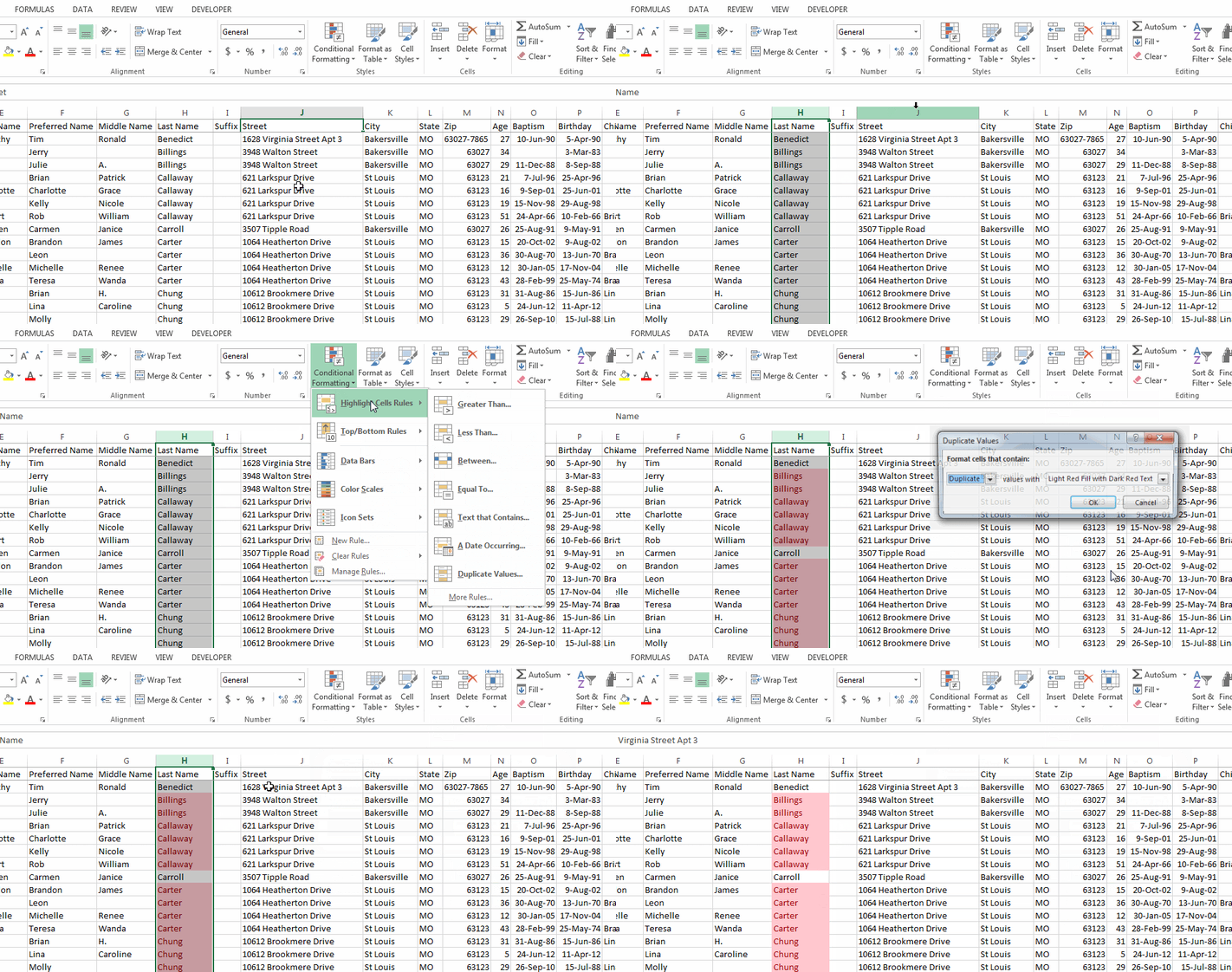
I use this the most to find duplicate values in a list of items. This makes it easier, for instance, to remove duplicate email addresses from a list.
To use Conditional Formatting in this way, highlight a column and go to Home > Conditional Formatting > Highlight Cell Rules > Duplicate Values.
4. Remove Duplicates
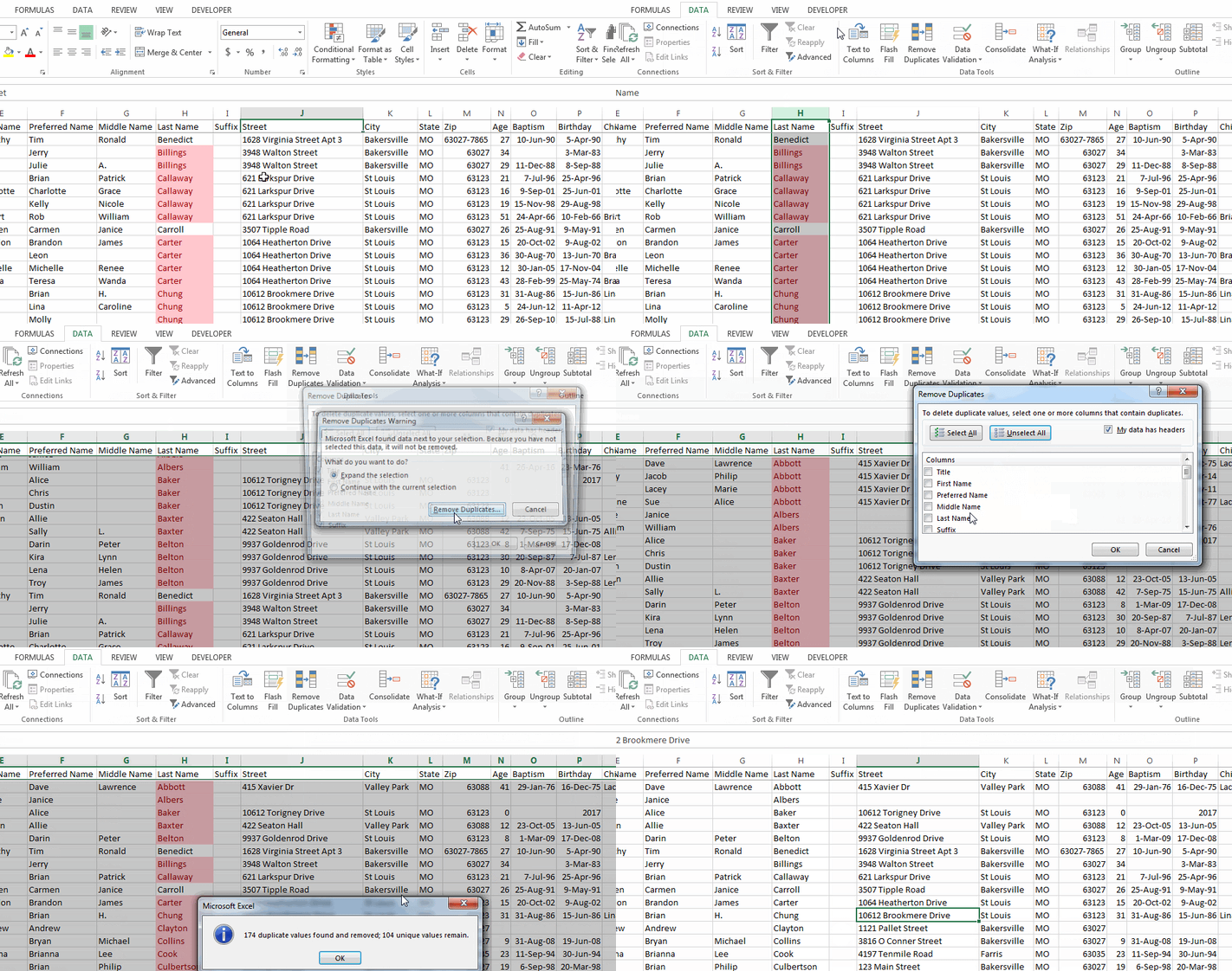
After you use Conditional Formatting to identify all the duplicate values, you could manually delete all duplicate entries. But there’s actually a tool that can automatically do this for you!
To use this tool, go to Data > Remove Duplicates and select the column(s) you want to remove duplicates from. Then click OK.
5. Sort By Color
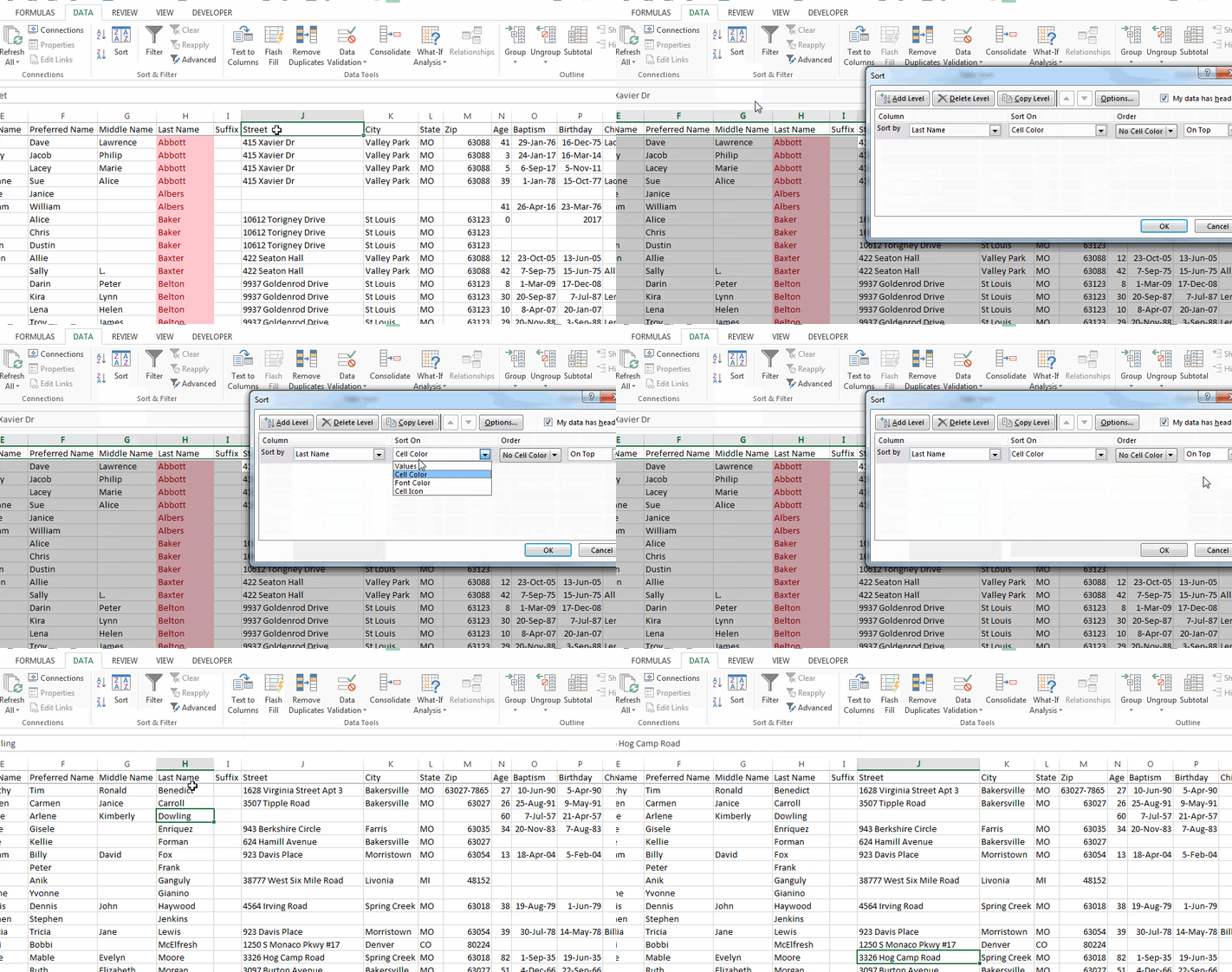
Many people know how to use the Sort tool to sort alphabetically or numerically, but did you know you could sort by formatting as well? For example, if you use Conditional Formatting to highlight duplicates, you can sort by color to put all unique values at the top of the spreadsheet and duplicate values at the bottom.
To use this tool, go to Data > Sort. Then choose which column to sort, which formatting feature to sort by, and what order to sort the data in, and click OK.
6. Text to Columns
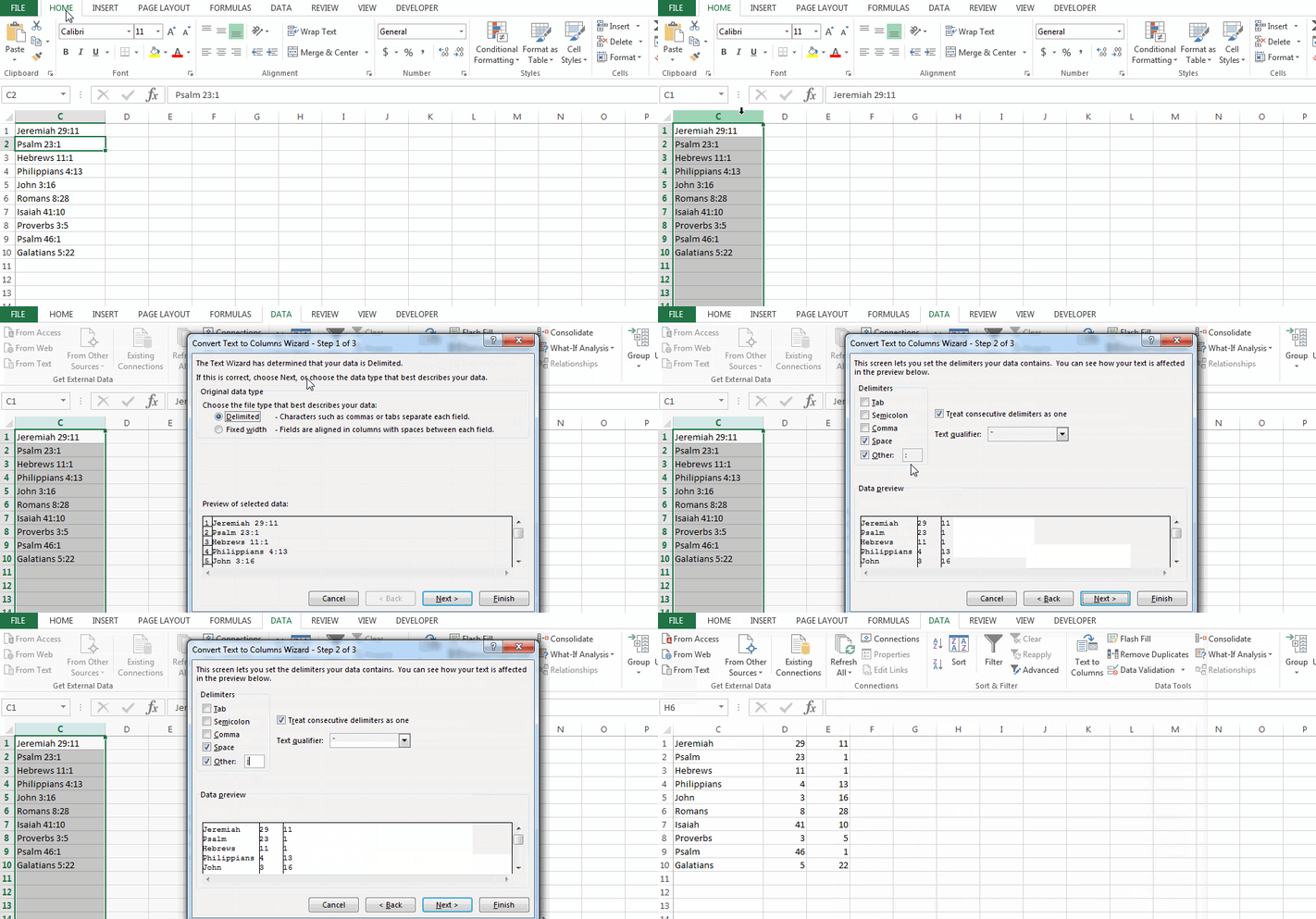
If you have a string of data in a single cell but you want to sort the data by something other than the cell’s first character, it can be quite frustrating. Rather than retyping everything, you can use Text to Columns to break that data down into a more usable format.
Text to Columns allows you to take the data in one column and break it apart into multiple columns. The tool looks at the characters inside the data to split it up. For example, with Bible verses, a space and a colon can be identified to consistently split up data.
To use this tool, first select the column with the data you want to break up. Then go to Data > Text to Columns, select Delimited, and click Next. Identify the delimiters you want to use (comma, colon, space, etc.) and click Finish. Now you can use these separate columns to sort your data however you need to.
7. Custom Lists for Sorting
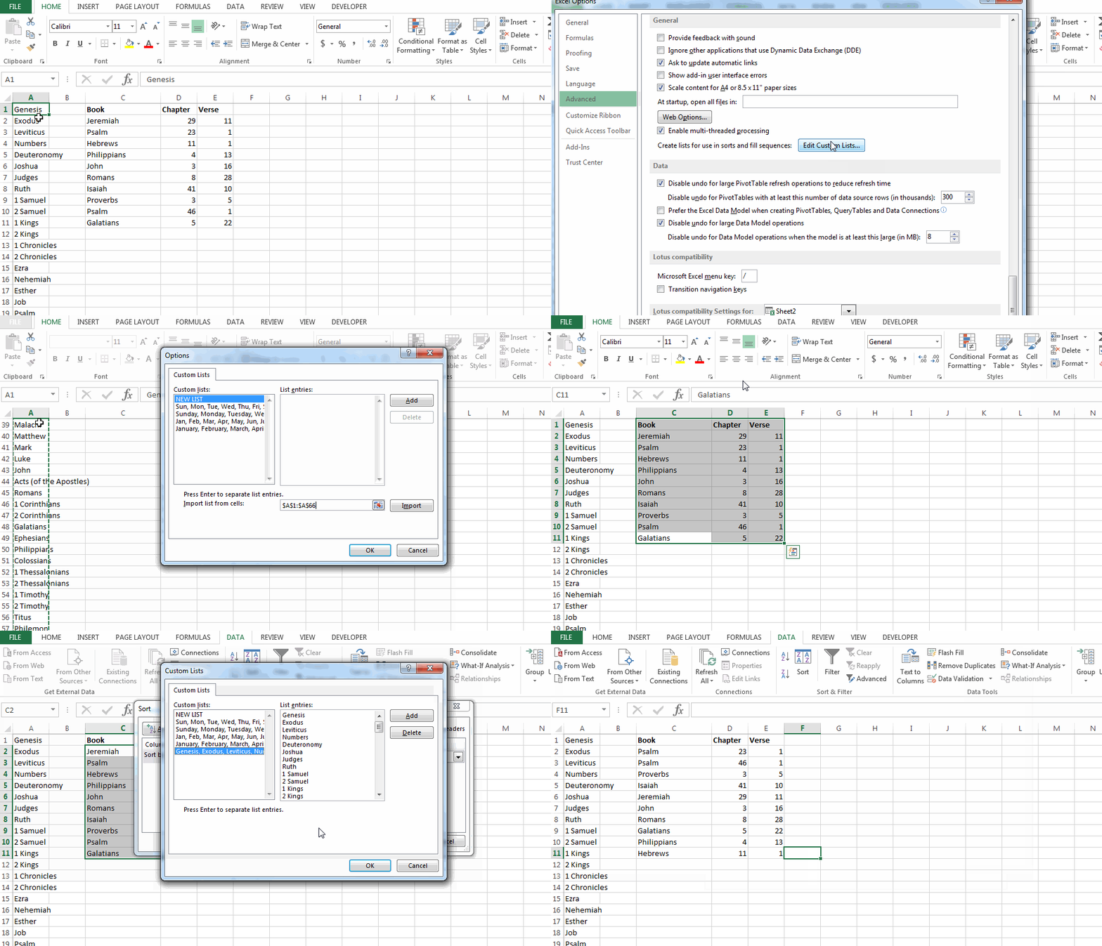
Sometimes you need to sort text not alphabetically. Maybe it’s for days of the week, months, or books of the Bible. This feature takes a bit more time to set up, but once you do it for a set of data, it’s really easy to use that data in the future.
To set this up, first go to File > Options > Advanced. Under General, click the button Edit Custom Lists. Enter your list, then click OK twice to get back to your data. Next, select the data you want to sort, and go to Data > Sort. Under Order, select Custom List. Select the custom list you want to use, and click OK twice to get back to your (now custom sorted) data.
These tricks just scratch the surface of what Excel is capable of doing, but I hope you find these tips useful. Finding quicker and easier ways to do data-entry tasks just means you can spend more time with people who need to hear the Gospel.
Learn more about the use of technology in your church by subscribing to this blog!
About the Author
Follow on Linkedin More Content by Peter Frank


